Configure Map Layout Data Plotting

Last Updated: July 2024

In this tutorial you will configure data plotting for your Tethys Map Layout that will allow users to click on features on your map and plot data associated with them.

../../_images/configure_data_plotting_solution.png

0. Start From Previous Solution (Optional)

If you wish to use the previous solution as a starting point:

git clone https://github.com/tethysplatform/tethysapp-map_layout_tutorial
cd tethysapp-map_layout_tutorial
git checkout -b add-spatial-data-solution add-spatial-data-solution-4.5

You'll also need to do the following:

Download the solution version of the sample NextGen data used in this tutorial: sample_nextgen_data_solution.zip.
Save to $TETHYS_HOME/workspaces/map_layout_tutorial/app_workspace
Unzip the contents to the same location
Delete the zip file
Rename the sample_nextgen_data_solution to sample_nextgen_data (i.e. remove "_solution")

1. Configure NextGen Data Plotting

We want to be able to wire up our application to easily explore and view the NextGen CSV outputs that we explored in a previous section. With the MapLayoutTutorialMap class we've been exploring, this is not too complicated.

To get basic plotting to work for the ouput NextGen data associated with the nexus points and catchments we've spatially added to our map, we simply need to override the get_plot_for_layer_feature function, copying its expected signatures (i.e. arguments) and returning the expected result. Let's take a look at what a functional, complete implementation will look like and then dive into the details.

Replace controller.py with the following:

import json
from pathlib import Path
import pandas as pd
from tethys_sdk.layouts import MapLayout
from tethys_sdk.routing import controller
from .app import App


MODEL_OUTPUT_FOLDER_NAME = 'sample_nextgen_data'

@controller(name="home", app_workspace=True)
class MapLayoutTutorialMap(MapLayout):
    app = App
    base_template = 'map_layout_tutorial/base.html'
    map_title = 'Map Layout Tutorial'
    map_subtitle = 'NOAA-OWP NextGen Model Outputs'
    default_map_extent = [-87.83371926334216, 33.73443611122197, -86.20833410475134, 34.456557011634175]
    max_zoom = 14
    min_zoom = 9
    show_properties_popup = True
    plot_slide_sheet = True

    def compose_layers(self, request, map_view, app_workspace, *args, **kwargs):
        """
        Add layers to the MapLayout and create associated layer group objects.
        """
        # Load GeoJSON from files
        config_directory = Path(app_workspace.path) / MODEL_OUTPUT_FOLDER_NAME / 'config'

        # Nexus Points
        nexus_path = config_directory / 'nexus_4326.geojson'
        with open(nexus_path) as nf:
            nexus_geojson = json.loads(nf.read())

        nexus_layer = self.build_geojson_layer(
            geojson=nexus_geojson,
            layer_name='nexus',
            layer_title='Nexus',
            layer_variable='nexus',
            visible=True,
            selectable=True,
            plottable=True,
        )

        # Catchments
        catchments_path = config_directory / 'catchments_4326.geojson'
        with open(catchments_path) as cf:
            catchments_geojson = json.loads(cf.read())

        catchments_layer = self.build_geojson_layer(
            geojson=catchments_geojson,
            layer_name='catchments',
            layer_title='Catchments',
            layer_variable='catchments',
            visible=True,
            selectable=True,
            plottable=True,
        )

        # Create layer groups
        layer_groups = [
            self.build_layer_group(
                id='nextgen-features',
                display_name='NextGen Features',
                layer_control='checkbox',  # 'checkbox' or 'radio'
                layers=[
                    nexus_layer,
                    catchments_layer,
                ]
            )
        ]

        return layer_groups

    @classmethod
    def get_vector_style_map(cls):
        return {
            'Point': {'ol.style.Style': {
                'image': {'ol.style.Circle': {
                    'radius': 5,
                    'fill': {'ol.style.Fill': {
                        'color': 'white',
                    }},
                    'stroke': {'ol.style.Stroke': {
                        'color': 'red',
                        'width': 3
                    }}
                }}
            }},
            'MultiPolygon': {'ol.style.Style': {
                'stroke': {'ol.style.Stroke': {
                    'color': 'navy',
                    'width': 3
                }},
                'fill': {'ol.style.Fill': {
                    'color': 'rgba(0, 25, 128, 0.1)'
                }}
            }},
        }

    def get_plot_for_layer_feature(self, request, layer_name, feature_id, layer_data, feature_props, app_workspace,
                                *args, **kwargs):
        """
        Retrieves plot data for given feature on given layer.

        Args:
            layer_name (str): Name/id of layer.
            feature_id (str): ID of feature.
            layer_data (dict): The MVLayer.data dictionary.
            feature_props (dict): The properties of the selected feature.

        Returns:
            str, list<dict>, dict: plot title, data series, and layout options, respectively.
        """
        output_directory = Path(app_workspace.path) / MODEL_OUTPUT_FOLDER_NAME / 'outputs'

        # Get the feature id
        id = feature_props.get('id')

        # Nexus
        if layer_name == 'nexus':
            layout = {
                'yaxis': {
                    'title': 'Streamflow (cfs)'
                }
            }

            output_path = output_directory / f'{id}_output.csv'
            if not output_path.exists():
                print(f'WARNING: no such file {output_path}')
                return f'No Data Found for Nexus "{id}"', [], layout

            # Parse with Pandas
            df = pd.read_csv(output_path)
            time_col = df.iloc[:, 1]
            streamflow_cms_col = df.iloc[:, 2]
            sreamflow_cfs_col = streamflow_cms_col * 35.314  # Convert to cfs
            data = [
                {
                    'name': 'Streamflow',
                    'mode': 'lines',
                    'x': time_col.tolist(),
                    'y': sreamflow_cfs_col.tolist(),
                    'line': {
                        'width': 2,
                        'color': 'blue'
                    }
                },
            ]

            return f'Streamflow at Nexus "{id}"', data, layout

        # Catchments
        else:
            layout = {
                'yaxis': {
                    'title': 'Evapotranspiration (mm/hr)'
                }
            }

            output_path = output_directory / f'{id}.csv'
            if not output_path.exists():
                print(f'WARNING: no such file {output_path}')
                return f'No Data Found for Catchment "{id}"', [], layout

            # Parse with Pandas
            df = pd.read_csv(output_path)
            data = [
                {
                    'name': 'Evapotranspiration',
                    'mode': 'lines',
                    'x': df.iloc[:, 1].tolist(),
                    'y': df.iloc[:, 2].tolist(),
                    'line': {
                        'width': 2,
                        'color': 'red'
                    }
                },
            ]

            return f'Evapotranspiration at Catchment "{id}"', data, layout

Let's take a closer look at what has changed.

There is a new import: pandas

This is the one third-party library that we added to our install.yml in the first section of this tutorial. We will need this package to read in and handle the CSV NextGen outputs.

A new constant is defined after the imports:

This references the folder within the app_workspace directory that serves as the root folder for the NextGen model output. This was changed to a constant since it will now be referenced in multiple places: both where the spatial data is accessed and now where the tabular data will be accessed.

Note that this constant is now used on the relevant line in the compose_layers function:

Two new properties are defined in the MapLayoutTutorialMap class:

class MapLayoutTutorialMap(MapLayout):
    ...
    ...
    ...
    show_properties_popup = True
    plot_slide_sheet = True

The must be explicitly defined since they default to False. Here's what they do:

show_properties_popup: Wires up a properties dialog that will now popup automatically when clicking on a feature and display the properties metadata associated with the feature as defined in the GeoJSON file. This will only apply to features that were configured with selectable = True, as we did with our NextGen layers in the last section.
plot_slide_sheet: Adds a Plot button to the properties dialog described in the line above and wire up the button to call the get_plot_for_features function when clicked (this function is discussed next). This will only apply to features that were configured with plottable = True, as we did with our NextGen layers in the last section.

With just those two lines added, the popup generated when clicking on a featuer will look like this:

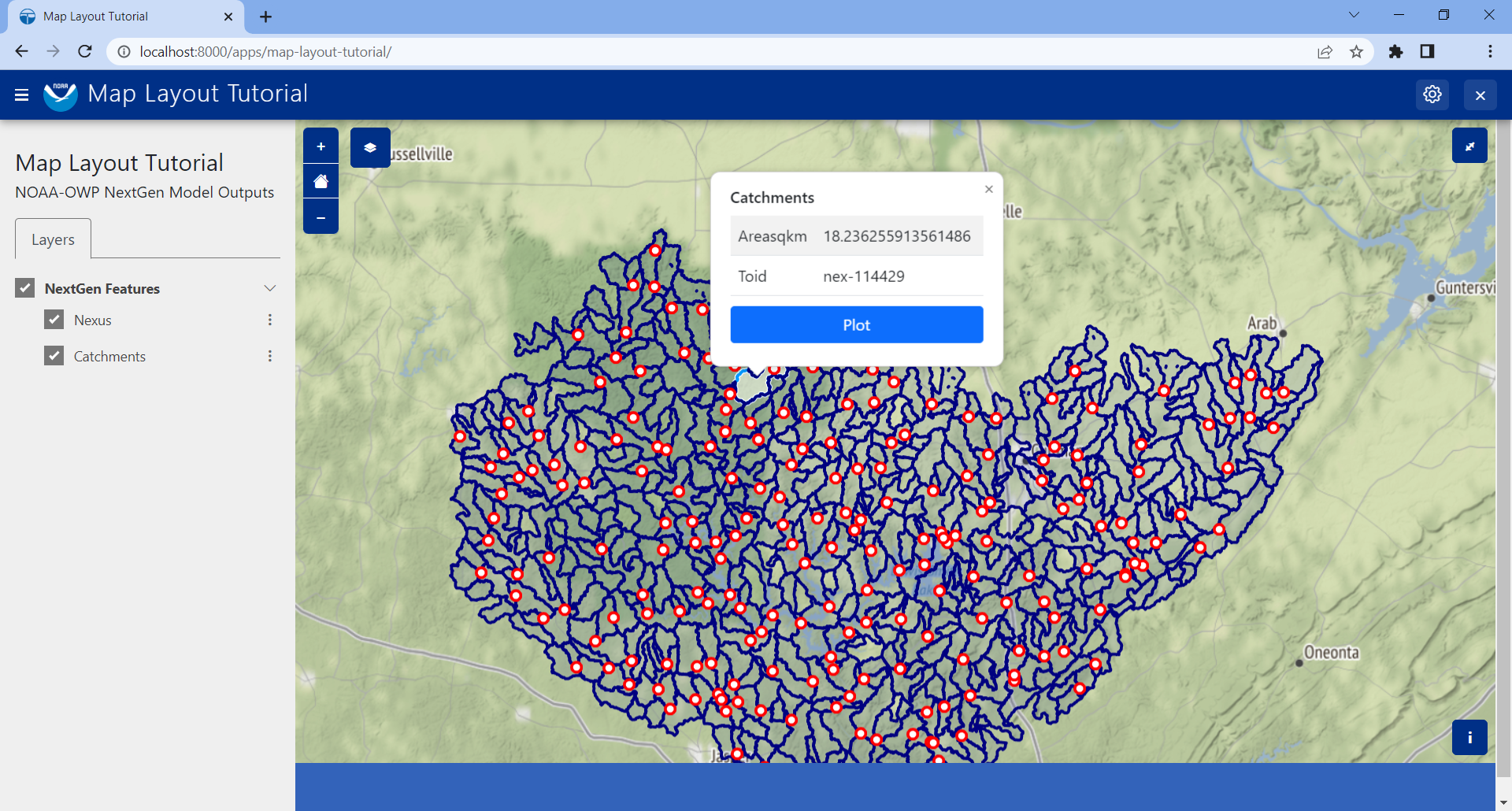
The get_plot_for_features function was added

Here's a closer look at that function:

def get_plot_for_layer_feature(self, request, layer_name, feature_id, layer_data, feature_props, app_workspace,
                                *args, **kwargs):
        """
        Retrieves plot data for given feature on given layer.

        Args:
            layer_name (str): Name/id of layer.
            feature_id (str): ID of feature.
            layer_data (dict): The MVLayer.data dictionary.
            feature_props (dict): The properties of the selected feature.

        Returns:
            str, list<dict>, dict: plot title, data series, and layout options, respectively.
        """
        output_directory = Path(app_workspace.path) / MODEL_OUTPUT_FOLDER_NAME / 'output'

        # Get the feature id
        id = feature_props.get('id')

        # Nexus
        if layer_name == 'nexus':
            layout = {
                'yaxis': {
                    'title': 'Streamflow (cfs)'
                }
            }

            output_path = output_directory / f'{id}_output.csv'
            if not output_path.exists():
                print(f'WARNING: no such file {output_path}')
                return f'No Data Found for Nexus "{id}"', [], layout

            # Parse with Pandas
            df = pd.read_csv(output_path)
            time_col = df.iloc[:, 1]
            streamflow_cms_col = df.iloc[:, 2]
            sreamflow_cfs_col = streamflow_cms_col * 35.314  # Convert to cfs
            data = [
                {
                    'name': 'Streamflow',
                    'mode': 'lines',
                    'x': time_col.tolist(),
                    'y': sreamflow_cfs_col.tolist(),
                    'line': {
                        'width': 2,
                        'color': 'blue'
                    }
                },
            ]

            return f'Streamflow at Nexus "{id}"', data, layout

        # Catchments
        else:
            layout = {
                'yaxis': {
                    'title': 'Evapotranspiration (mm/hr)'
                }
            }

            output_path = output_directory / f'{id}.csv'
            if not output_path.exists():
                print(f'WARNING: no such file {output_path}')
                return f'No Data Found for Catchment "{id}"', [], layout

            # Parse with Pandas
            df = pd.read_csv(output_path)
            data = [
                {
                    'name': 'Evapotranspiration',
                    'mode': 'lines',
                    'x': df.iloc[:, 1].tolist(),
                    'y': df.iloc[:, 2].tolist(),
                    'line': {
                        'width': 2,
                        'color': 'red'
                    }
                },
            ]

            return f'Evapotranspiration at Catchment "{id}"', data, layout

This function is passed six standard arguments: request, layer_name, feature_id, layer_data, feature_props, and app_workspace. In our case, we only need to use the layer_name, feature_props, and app_workspace variable. We'll describe how each is used as we explore what this function does.

This function does the following:

Composes the path to the outputs folder where our NextGen tabular (CSV) data is stored. Note the use of the MODEL_OUTPUT_FOLDER_NAME constant.
Uses the feature_props argument (that is passed in when the Plot button is clicked) to extract the id of the specific feature clicked. This comes from the properties metadata associated with the feature as defined in the GeoJSON file.
Uses the layer_name argument to distinguish between the "nexus" and "catchment" layers. This will match the same value chosen when configuring the layer with the build_geojson_layer function, as we did in the previous section.
For each layer, whether "nexus" or "catchment", the code handles the following:
1. Define the layout variable - one of the expected return values - which in this case is used only to define the y-axis label.
2. Compose the exact path to the selected feature's corresponding tabular data. For nexus data it should be a file named <nexID>_output.csv and for catchment data it should be a file named <catID>.csv as was discovered and discussed in the Data Prep section.
3. Check if the tabular file actually exists, and if not return an appropriate message (i.e. chart title), data (in this case, none or []), and the defined layout.
4. If the file exists, it is opened using the read_csv method of pandas
5. Then, the separate columns of data that are desired for the plot axes are separated out into distinct variables using the iloc accessor of pandas, where the provided integer represents the 0-based column number. These can be confirmed by manually opening inspecting the CSV files. For the nexus data, we want "Time" (column 1) on the x-axis and Streamflow (column 2) on the y-axis. Note that we also convert Streamflow from CMS to CFS. For the catchment data, we want "Time" (column 1) on the x-axis and Evapotranspiration (column 2)
6. The structured data variable is composed: a dictionary with the following keys: name, mode, x, y, and line, where line has its own dictionary defining its width and color. These values can be played with to achieve the look and feel that you desire.
7. Finally, the expected data is returned: the title of the plot, the data to plot (data variable) and the plot display properties (layout)

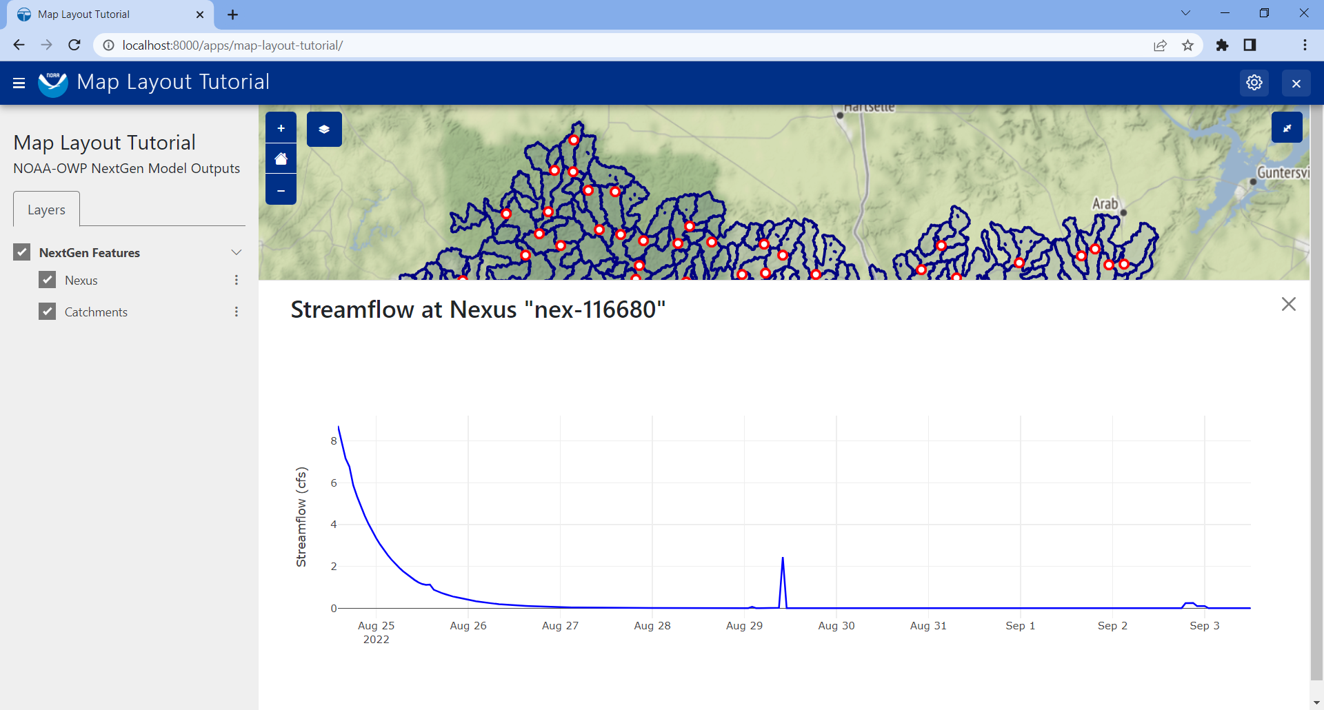
With this code all wired up, you can now click the Plot button on the popup for any feature, and assuming the tabular data exists for that feature (and it should), then a plot will slide into view that displays the corresponding model output data for that feature. It should look something like the figure at the top of this section.

There you have it! With less than 200 lines of code, we have quickly developed a useful data viewer for the NextGen model.

5. Solution

This concludes the Configure Data Plotting portion of the Map Layout Tutorial. You can view the solution on GitHub at https://github.com/tethysplatform/tethysapp-map_layout_tutorial/tree/configure-data-plotting-solution or clone it as follows:

git clone https://github.com/tethysplatform/tethysapp-map_layout_tutorial
cd tethysapp-map_layout_tutorial
git checkout -b configure-data-plotting-solution configure-data-plotting-solution-4.5

You'll also need to do the following:

Download the solution version of the sample NextGen data used in this tutorial: sample_nextgen_data_solution.zip.
Save to tethysapp-map_layout_tutorial/tethysapp/map_layout_tutorial/workspaces/app_workspace
Unzip the contents to the same location
Delete the zip file
Rename the sample_nextgen_data_solution to sample_nextgen_data (i.e. remove "_solution")

Add Spatial Data to Map Layout

Additional Exercises